Time Series Forecasting Experiments: Classical vs Machine Learning Approaches

A hands-on exploration comparing classical statistical methods (ARIMA, decomposition) with modern machine learning algorithms for forecasting air passenger traffic.

Introduction

Time series forecasting is a fundamental problem in data science, with applications ranging from demand prediction to financial market analysis. But which approach works best? Classical statistical methods like ARIMA have been the gold standard for decades, while machine learning algorithms promise greater flexibility and performance.

In the summer of 2024, I set out to answer this question through hands-on experimentation. Using real-world air passenger traffic data, I compared three distinct methodologies: classical decomposition, ARIMA modeling, and machine learning algorithms. This project became a practical laboratory for understanding how different techniques handle temporal patterns, trends, and seasonality.

Table of Contents

1. The Dataset
2. Understanding the Data: Decomposition
3. Testing for Stationarity
4. Experimental Approaches
5. Results and Comparison
6. Key Insights
7. Conclusion

The Dataset

I worked with monthly US air passenger traffic data, focusing on a specific time window:

• Training Period: 2016-2018 (monthly aggregated data)
• Test Period: 2019 (first 6 months)
• Target Variable: Total passenger count

The dataset provided a rich playground for experimentation—it exhibits clear seasonality (people travel more during summer and holidays), an upward trend (growing air traffic over time), and enough complexity to challenge different modeling approaches.

Understanding the Data: Decomposition

Before diving into predictions, I needed to understand what I was dealing with. Time series decomposition breaks down a series into three fundamental components:

1. Trend: The long-term progression (are passenger numbers generally increasing or decreasing?)
2. Seasonality: Regular patterns that repeat over fixed periods (summer peaks, winter dips)
3. Residual: Random noise that can't be explained by trend or seasonality

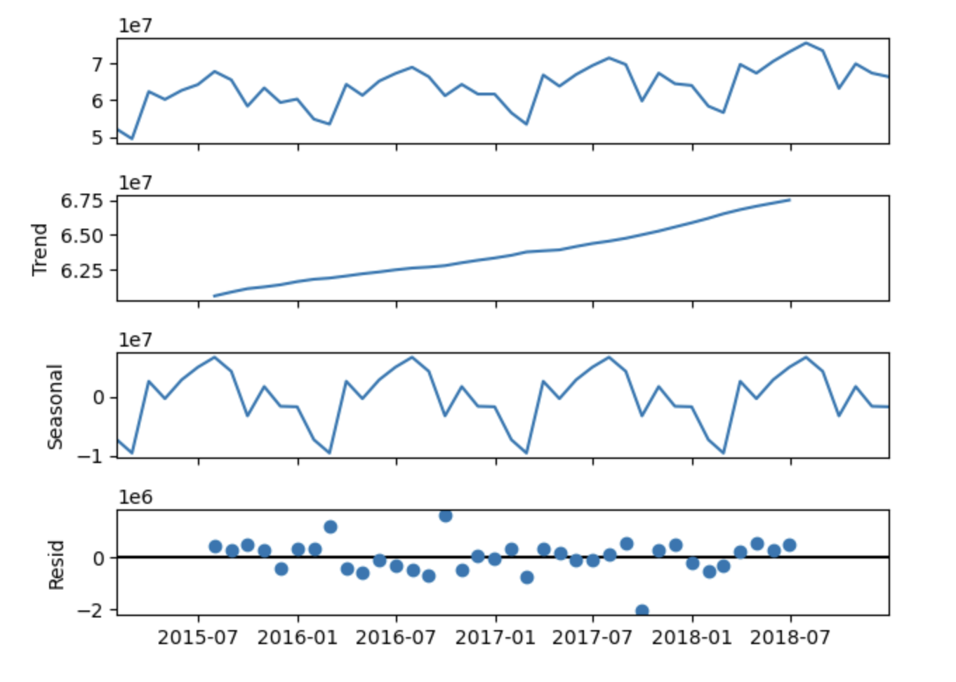Figure 1: Decomposition of passenger traffic into trend, seasonal, and residual components

This decomposition immediately revealed:

• A clear upward trend in passenger numbers from 2016 to 2018
• Strong seasonal patterns with predictable peaks and valleys
• Relatively small residuals, suggesting the trend and seasonality capture most of the variation

Testing for Stationarity

A critical concept in time series analysis is stationarity—whether the statistical properties of the series remain constant over time. Many classical methods, including ARIMA, assume or require stationarity.

I used the Augmented Dickey-Fuller (ADF) test to check for stationarity. The test revealed that the original series was non-stationary due to the trend component. This finding guided my modeling approach, particularly for ARIMA, where I needed to account for this non-stationarity.

ACF and PACF Analysis

To better understand the temporal structure of the data, I examined the autocorrelation function (ACF) and partial autocorrelation function (PACF):

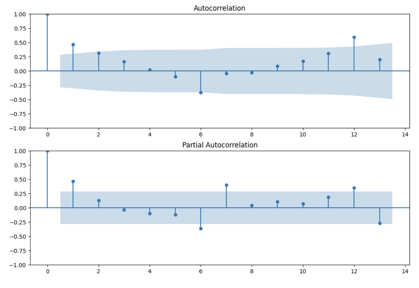Figure 2: Autocorrelation (ACF) and Partial Autocorrelation (PACF) plots

These plots helped identify:

• The presence of strong autocorrelation at multiple lags
• Seasonal patterns evident in the periodic spikes
• Appropriate ARIMA parameters for modeling

Experimental Approaches

I tested three distinct methodologies, each with its own strengths and assumptions:

Approach 1: Trend + Seasonality Decomposition

The simplest approach: Use linear regression to model and extrapolate the trend, then add back the historical seasonal patterns.

Pros:

• Highly interpretable—you can literally see what drives your predictions
• Fast to compute
• Works well when patterns are stable

Cons:

• Assumes the future looks like the past (linear trend continuation)
• No ability to capture non-linear relationships
• Vulnerable to sudden changes in patterns

Approach 2: ARIMA Modeling

The classical statistical approach: ARIMA (AutoRegressive Integrated Moving Average) models the series as a combination of its own past values, past errors, and differencing to handle non-stationarity.

I used Auto ARIMA to select optimal parameters, which identified ARIMA(2,0,2) as the best model for the detrended series. The trend component was added back to generate final predictions.

Pros:

• Grounded in solid statistical theory
• Handles temporal dependencies explicitly
• Well-studied with known properties

Cons:

• Requires careful parameter selection
• Assumes linear relationships
• Can struggle with complex seasonal patterns

Approach 3: Machine Learning

The modern approach: Treat time series forecasting as a supervised learning problem by creating features from past observations (lag features, rolling statistics, etc.).

I tested four algorithms:

• Linear Regression: Baseline ML approach
• Random Forest Regressor: Ensemble method capturing non-linear patterns
• Support Vector Regressor (SVR): Kernel-based method
• XGBoost Regressor: Gradient boosting for complex interactions

Pros:

• Can capture non-linear relationships
• Easy to incorporate external features (weather, holidays, etc.)
• No stationarity assumptions

Cons:

• Less interpretable
• Requires careful feature engineering
• Risk of overfitting without proper validation

Results and Comparison

After training all models on 2016-2018 data, I evaluated their performance on the 2019 test period using Root Mean Squared Error (RMSE) as the metric.

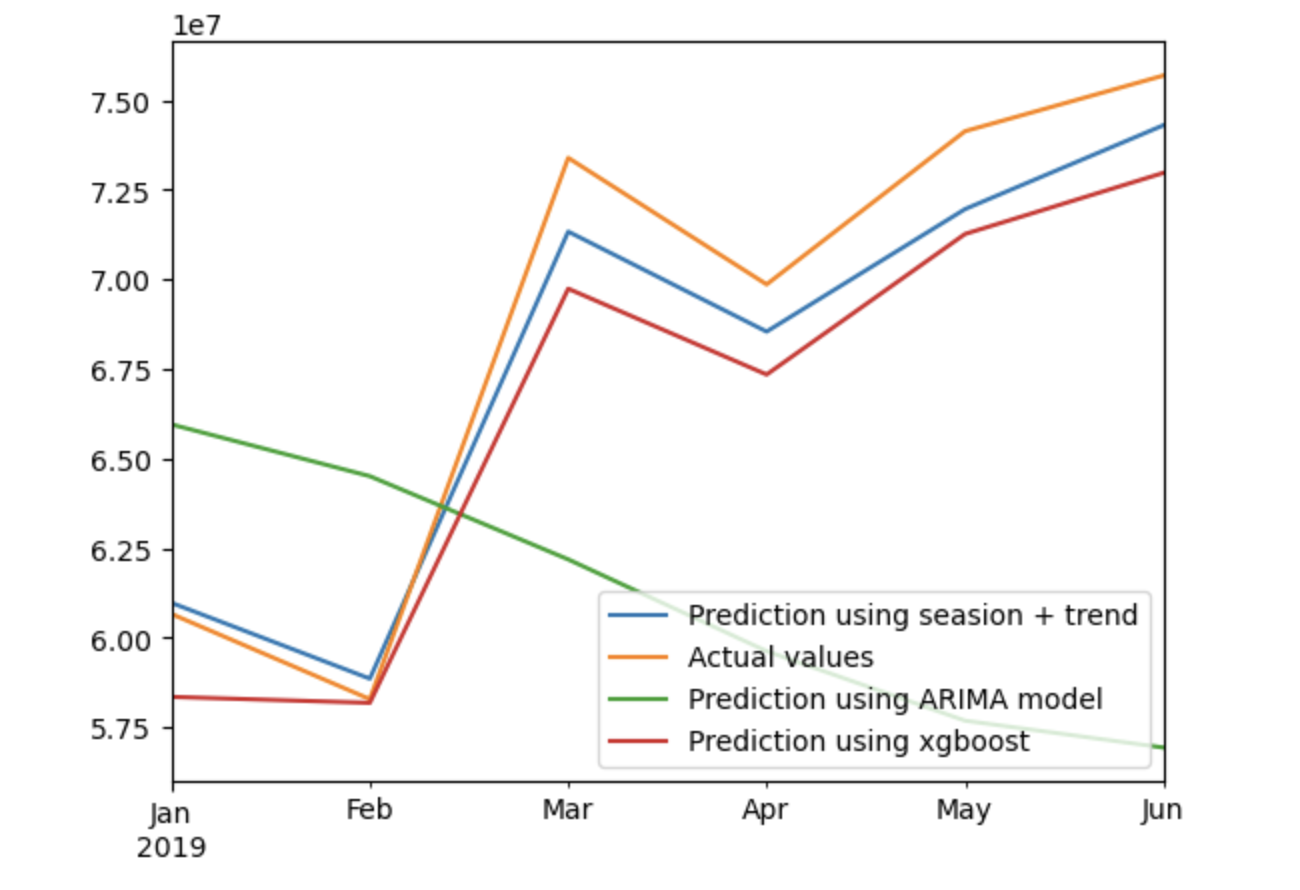Figure 3: Comparison of predicted vs actual passenger counts for 2019

Key Insights

Through this experimentation, several important lessons emerged:

1. Simple Can Be Powerful

Classical decomposition, despite its simplicity, performed surprisingly well. When your data has clear, stable patterns, sophisticated methods don't always win.

2. Domain Knowledge Matters

Understanding your data through decomposition and stationarity tests isn't just academic—it directly informs which methods will work best.

3. ML Flexibility Comes with Trade-offs

Machine learning models offered flexibility but required more careful feature engineering and validation. They didn't automatically outperform simpler methods.

4. Evaluation is Everything

RMSE provided a clear, quantitative comparison, but visual inspection of predictions vs. actuals revealed insights that metrics alone couldn't capture.

Conclusion

Time series forecasting isn't about finding the "one best method"—it's about understanding your data and matching the right tool to the problem. Classical methods like ARIMA and decomposition remain powerful when data exhibits clear patterns, while machine learning opens doors to incorporating complex features and non-linear relationships.

This experimental approach taught me that hands-on comparison beats theoretical debates. By implementing multiple methods side-by-side, I gained intuition that no textbook could provide about how different techniques handle real-world temporal data.

Whether you're predicting passenger traffic, sales forecasts, or stock prices, the principles remain the same: understand your data, test multiple approaches, and let the results guide your decisions.

Repository: View on GitHub